Optimizing Convolutions
A common operation in graphics is to apply a convolution to an image; that is, for each pixel in the output, perform a weighted sum of the input pixel’s neighborhood. The neighborhood weights in this case are known as a convolution kernel. The simplest convolution kernel is a box filter, where all the weights are 1:
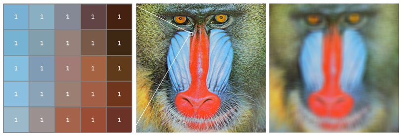
So, for a kernel of width N and an image size of W*H pixels, the convolution requires (N*N)*(W*H) texture fetches. This will quickly become impractically slow for realtime use - at 1080p even a small 5x5 kernel would require 51,840,000 texture fetches…yikes.
Separability
Some kernels are separable, which means that the matrix of weights can be expressed as the outer product of two vectors:
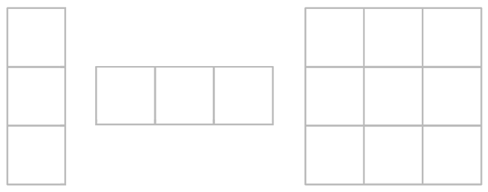
Separable kernels are useful computationally because a convolution by an N*N kernel can be split into 2 successive convolutions by an N*1 and 1*N kernel (a horizontal pass followed by a vertical pass). That’s (N*W*H)+(N*W*H) texture fetches which is significantly more manageable - 20,736,000 fetches for a 5x5 kernel at 1080p.
Note that this works because convolution is associative: x * (N * N) == (x * N) * N.
Bilinear Filtering
A common trick is to exploit hardware texture filtering to combine adjacent pairs (or quads for the 2d case) of texture fetches into one bilinear sample:
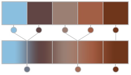
This reduces the kernel width to N / 2 + 1. Note that for this to work we must modify the kernel weights and the offsets used to sample the input texture. If we consider a pair of texture fetches at offsets o1 and o2 with their respective weights:
t[o1] * w1 + t[o2] * w2
The combined weight for both samples w3 is the sum of the individual weights:
w3 = w1 + w2
The offset can then be computed in terms of the weights:
o3 = (o1 * w1 + o2 * w2) / w3
This is basically lerping between the two sample offsets with respect to the weights. I provide code for computing the weights and offsets for 1d or 2d kernels in Appendix A (and the sample project).
This reduces the kernel width to N / 2 + 1, bringing us down to 12,441,600 texture fetches for a 5x5 kernel at 1080p. While this is a practical optimization for small, simple convolutions, it doesn’t work for more complicated operations which require dynamic weights (such as bilateral filters).
Cached Texture Fetches
Suppose we’re using a compute shader to perform the convolution. Within each thread group, the convolution kernels overlap such that most of the texture fetches are redundant:
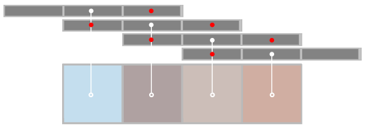
For each center tap (white dots), adjacent kernels overlap and perform redundant taps (red dots).
We can eliminate this redundancy by using group shared memory to cache texture reads. A basic implementation needs to load an additional N - 1 samples at the borders of the group:

The convolution can then be performed using shared memory access instead of texture fetches.
For a separable 5x5 kernel at 1080p this approach takes 2,479,680 texture fetches (with 64 threads per group). Careful consideration needs to be taken to achieve peak performance and eliminate redundant threads - see (1) and the sample project for details.
Prefiltering
So far we have discussed optimizations which are appropriate for convolutions over a relatively small spatial domain. However one of the most important use cases for convolution is to blur an image, and in this case we very frequently want a perceptually large blur with good performance but without necessarily being an accurate Gaussian convolution.
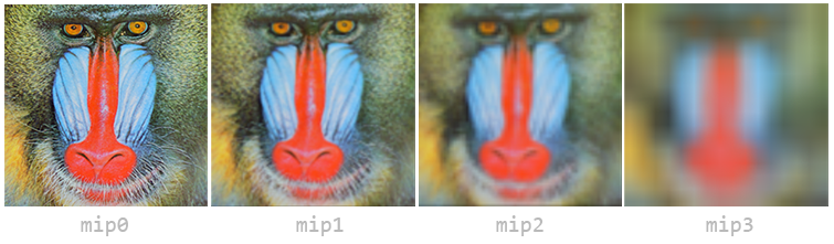
The core idea is to prefilter the image by applying a small convolution successively into the mip chain of the source image. This could be as simple as a box filter:
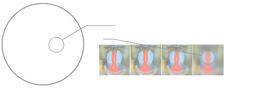
We can then resample the prefiltered mipmap to approximate a large blur using a fixed number of samples. For example we could use a Poisson disk and calculating the area under each sample to select a mip whose texels cover a similar area:
Randomly rotating the sample kernel trades banding for noise, which can be trivially removed by temporal supersampling (basically for free if you already have temporal antialiasing). See the bonus slides of (4) for a wealth of information, particular ‘interleaved gradient noise’.
Note that with the improved texture cache efficiency of sampling smaller mips, the actual performance of this approach is close to constant with a varying blur radius.
References
- DirectCompute Accelerated Separable Filters (AMD)
- Bicubic Filtering in Fewer Taps (Phill Djonov)
- The Gaussian Kernel (Moo K. Chung)
- Next Generation Post Processing in Call of Duty: Advanced Warfare (Jorge Jimenez)
Appendix A - Bilinear Optimization Code
The two functions below take an existing kernel and generate an optimized version for bilinear texture filtering.
// Outputs are arrays of _width / 2 + 1.
void KernelOptimizeBilinear1d(int _width, const float* _weightsIn, float* weightsOut_, float* offsetsOut_)
{
	const int halfWidth = _width / 2;
	int j = 0;
	for (int i = 0; i != _width - 1; i += 2, ++j)
	{
		float w1 = _weightsIn[i];
		float w2 = _weightsIn[i + 1];
		float w3 = w1 + w2;
		float o1 = (float)(i - halfWidth);
		float o2 = (float)(i - halfWidth + 1);
		float o3 = (o1 * w1 + o2 * w2) / w3;
		weightsOut_[j] = w3;
		offsetsOut_[j] = o3;
	}
	weightsOut_[j] = _weightsIn[_width - 1];
	offsetsOut_[j] = (float)(_width - halfWidth - 1);
}
// Outputs are arrays of (_width / 2 + 1) ^ 2.
void KernelOptimizeBilinear2d(int _width, const float* _weightsIn, float* weightsOut_, vec2* offsetsOut_)
{
const int outWidth = _width / 2 + 1;
const int halfWidth = _width / 2;
int row, col;
for (row = 0; row < _width - 1; row += 2)
{
for (col = 0; col < _width - 1; col += 2)
{
float w1 = _weightsIn[(row * _width) + col];
float w2 = _weightsIn[(row * _width) + col + 1];
float w3 = _weightsIn[((row + 1) * _width) + col];
float w4 = _weightsIn[((row + 1) * _width) + col + 1];
float w5 = w1 + w2 + w3 + w4;
float x1 = (float)(col - halfWidth);
float x2 = (float)(col - halfWidth + 1);
float x3 = (x1 * w1 + x2 * w2) / (w1 + w2);
float y1 = (float)(row - halfWidth);
float y2 = (float)(row - halfWidth + 1);
float y3 = (y1 * w1 + y2 * w3) / (w1 + w3);
const int k = (row / 2) * outWidth + (col / 2);
weightsOut_[k] = w5;
offsetsOut_[k] = vec2(x3, y3);
}
float w1 = _weightsIn[(row * _width) + col];
float w2 = _weightsIn[((row + 1) * _width) + col];
float w3 = w1 + w2;
float y1 = (float)(row - halfWidth);
float y2 = (float)(row - halfWidth + 1);
float y3 = (y1 * w1 + y2 * w2) / w3;
const int k = (row / 2) * outWidth + (col / 2);
weightsOut_[k] = w3;
offsetsOut_[k] = vec2((float)(col - halfWidth), y3);
}
for (col = 0; col < _width - 1; col += 2)
{
float w1 = _weightsIn[(row * _width) + col];
float w2 = _weightsIn[(row * _width) + col + 1];
float w3 = w1 + w2;
float x1 = (float)(col - halfWidth);
float x2 = (float)(col - halfWidth + 1);
float x3 = (x1 * w1 + x2 * w2) / w3;
const int k = (row / 2) * outWidth + (col / 2);
weightsOut_[k] = w3;
offsetsOut_[k] = vec2(x3, (float)(row - halfWidth));
}
const int k = (row / 2) * outWidth + (col / 2);
weightsOut_[k] = _weightsIn[(row * _width) + col];
offsetsOut_[k] = vec2(_width / 2, _width / 2);
}Appendix B - Computing Gaussian Weights
Theo Mader has a very nifty web-based Gaussian weights calculator here. I’ve also provided some C code for generating Gaussian and binomial kernels in the sample project.
An interesting point to note about Gaussian kernels is the standard deviation parameter sigma (σ). It’s easiest to understand this parameter by looking at how different values affect the Gaussian distribution:
The spatial domain of the Gaussian function is infinite, but we truncate it to our finite kernel size. Sigma is therefore important in order to correctly tune the distribution of weights within the kernel; the ideal sigma should be chosen such that the weights at the kernel’s boundary are the smallest nonzero weights for a given precision (e.g. 1/255 for an 8-bit image). Using a value of sigma larger than the ideal value produces a perceptually bigger blur but converges to a box filter. Using a smaller value than the ideal wastes samples because some of the kernel weights are effectively zero.