Dynamic Local Exposure

In this post I’ll present some ideas about managing dynamic local exposure for HDR rendering. Bart Wronski already has an excellent post on this subject and I strongly recommend reading it now if you haven’t already; the ideas here are based largely on information in his post. I’ve included some other great references at the end.

Low/High Dynamic Range

Back in the good ol’ days (the 1990s), games were rendered directly in a displayable, low dynamic range format (gamma space, 8-bit). This was simple and cheap, but on the other hand presented a significant barrier to generating really photorealistic images (5).

Nowadays, especially with the advent of physically-based lighting, games are rendered with huge dynamic range, in linear space at higher precision. With this move towards photorealism comes a real-world problem: how do we map a high dynamic range image for a low dynamic range display?

Global Auto Exposure

The standard approach for automated exposure control is to measure the average (or log average) scene luminance, optionally with a weighting function to prefer values towards the image center. This can be done very efficiently via a parallel reduction, or by repeatedly downsampling into the mipmap of the luminance buffer. The latter approach has some advantages, which I’ll cover in the next section.

The average luminance is subsequently converted into an exposure scale, for example by computing the reciprocal of the maximum allowable scene luminance:

float Lavg = exp(textureLod(txLuminance, uv, 99.0).x);
float ev100 = log2(Lavg * 100.0 / 12.5);
ev100 -= uExposureCompensation; // optional manual bias 
float exposure = 1.0 / (1.2 * exp2(ev100));

This is derived from the ISO standard for computing saturation-based speed, see (3) for a complete explanation.

Because the average luminance is potentially unstable under dynamic conditions, it is common to smooth it over time via an exponential hysteresis function (2):

Lavg = Lavg + (Lnew - Lavg) * (1.0 - exp(uDeltaTime * -uRate));

Due it’s global nature, this approach suffers from areas of the image being under- or over-exposed, where there is deviation from the average luminance:

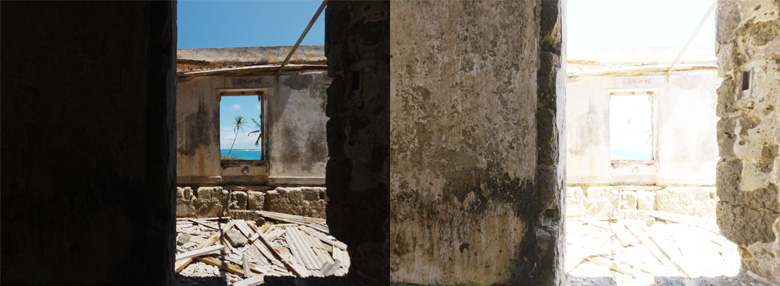
While this matches the eye’s ability to adapt to changing light levels, the overall effect is quite far from what we can actually perceive in the real world.

Local Auto Exposure

If we generated the average luminance by repeated downsampling, we can access lower mip levels of the luminance buffer to get a local average luminance (4).

float Lavg = exp(textureLod(txLuminance, uv, uLuminanceLod).x;

Note that for this to work, the hysteresis should only be applied at the last step (when writing the 1x1 mip level), otherwise there will be ghosting.

In theory this is a great idea: each area of the image can be well-exposed while still preserving contrast between adjacent areas. In practice, though, you get a hideous mess:

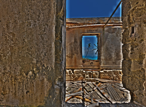
Most objectionable are the blocky ‘halos’ which occur in regions of high contrast:

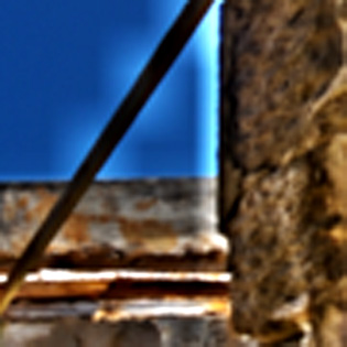
However these can be softened, either by prefiltering the luminance buffer or simply via bicubic sampling:

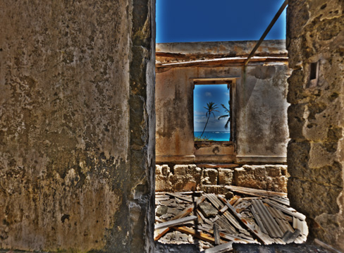
Still hideous, but less pixelated.

Sampling different levels of the luminance mipmap controls the halo radius. This is a useful parameter to control the overall ‘look’ of the result, as well as minimize the halo effect, albeit at the cost of either reducing the overall contrast (it becomes an edge filter) or losing the locality of the exposure control:

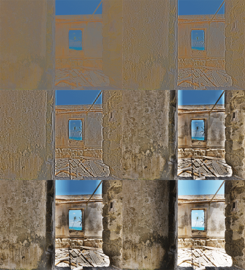
Softening the halos isn’t enough, though. The result is not at all natural; it’s the extreme ‘HDR photo’ style rather than human vision. However by blending between the global and local value, we can have the best of both worlds:

float Llocal  = exp(textureLod(txLuminance, uv, uLuminanceLod).x;
float Lglobal = exp(textureLod(txLuminance, uv, 99.0).x;
float L       = mix(Lglobal, Llocal, uLocalExposureRatio);
// .. use L to compute the final exposure scale as before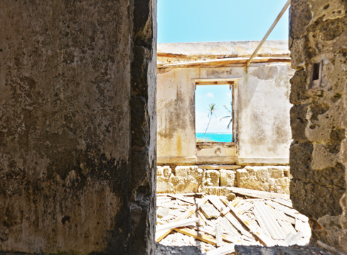

By modifying the blend ratio, the local exposure can be tuned to minimize artefacts and maximize the perceptual realism of the result:

Automated Blend Ratio

Tuning the blend ratio by hand is ok for situations with absolute control over the camera position, lighting, etc. However there are a lot of cases (e.g. outdoor games with dynamic time of day) where this level of control simply isn’t possible. Here it would be nice to generate the blend ratio automatically by detecting when it is most required.

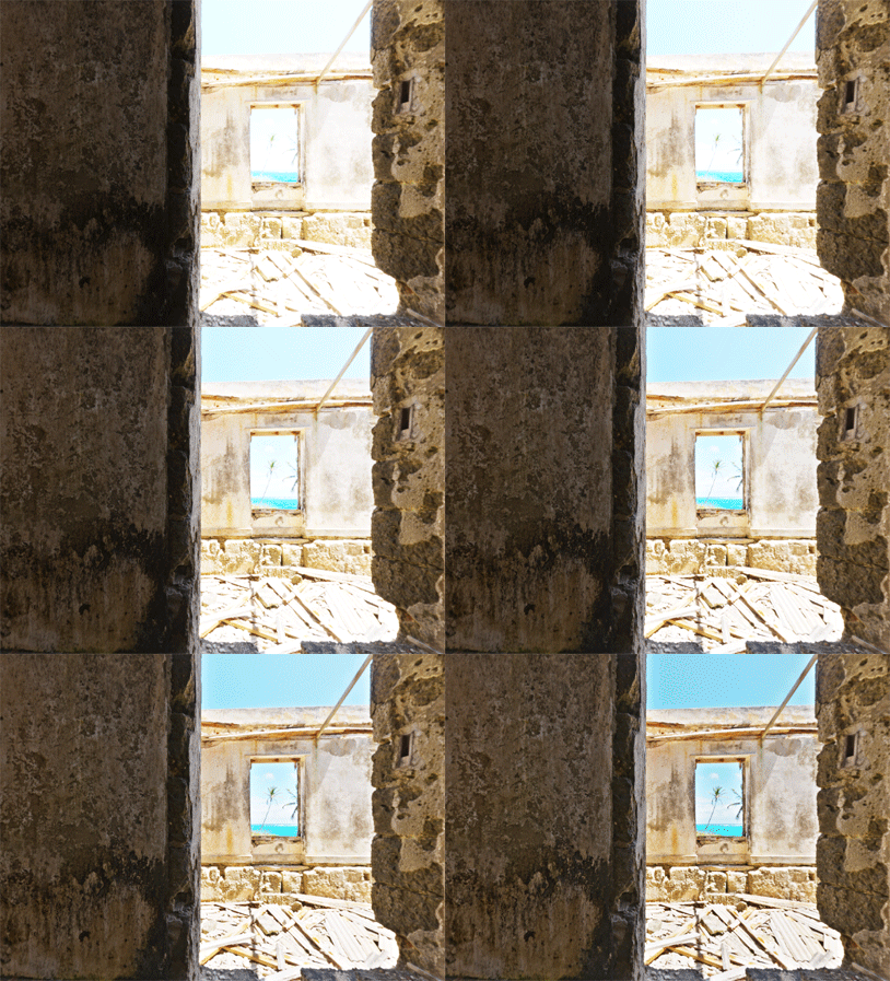
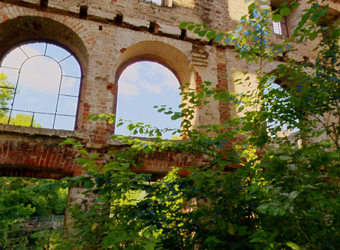
In the image below we have a wide dynamic range; mainly mid-to-low luminance values with a few very high intensity regions (the sky through the windows):

Without local exposure, the sky color is lost. In this case we’d like the blend ratio to be high:

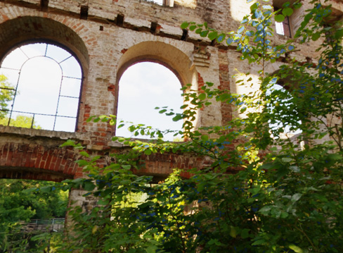
Now consider the image below, which contains a narrower dynamic range with mainly high luminance:

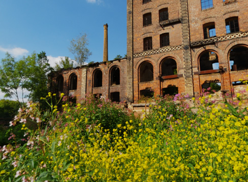
In this case, applying local exposure tends to squash the bright areas too much:

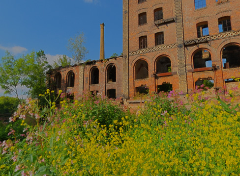
These observations hint at a simple heuristic for automating the local/global blend: as the difference between the average and maximum scene luminance increases, so the local exposure blend ratio should increase. Generating the maximum scene luminance can be done trivially during luminance metering, applying hysteresis to smooth the result in the same way as for the average. We can then extend the previous code snippet as follows:

float Llocal  = exp(textureLod(txLuminance, uv, uLuminanceLod).x;
float Lglobal = exp(textureLod(txLuminance, uv, 99.0).x; // average in x
float Lmax    = exp(textureLod(txLuminance, uv, 99.0).y; // max in y
float Lratio  = min(saturate(abs(Lmax - Lglobal) / Lmax), uLocalExposureMax);
float L       = mix(Lglobal, Llocal, Lratio);
// .. use L to compute the final exposure scale as before

Note that we now have uLocalExposureMax as an input to control the absolute maximum amount of local exposure to apply. I’ve found good results with uLocalExposureMax < 0.3.

Conclusion

The approach I outlined above imposes some constraints on when to measure the scene luminance. It is common to perform metering immediately after the lighting pass so as to avoid adapting to particle effects, bloom etc. However, when using the local luminance it is important that the actual value being exposed is represented in the luminance map. This means that metering needs to happen immediately before the exposure is applied. If this isn’t acceptable, a solution would be to generate the local luminance separately to the average/max.

While I think that exploiting both local and global information about the scene luminance is the ‘right’ approach to generating a balanced, natural-looking image, the quality of the result is obviously subjective. Whether or not a system like this fits a particular game depends entirely on the content and the desired visual style. I’d be interested to hear other ideas for doing this.

References

1. Localized Tonemapping (Bart Wronski)
2. Implementing a Physically Based Camera (Padraic Hennessy)
3. Moving Frostbite to PBR (Sébastien Lagarde, et al.)
4. A Closer Look at Tonemapping (Matt Pettineo)
5. The Importance of Being Linear (Larry Gritz, et al.)
6. Advanced Techniques and Optimization of HDR/VDR Color Pipelines (Timothy Lottes)

The HDR images used in the screenshots are from the sIBL Archive.